kdensity
Kernel Density Estimation with Parametric Starts and Asymmetric Kernels
Handles univariate non-parametric density estimation with
parametric starts and asymmetric kernels in a simple and flexible way.
Kernel density estimation with parametric starts involves fitting a
parametric density to the data before making a correction with kernel
density estimation, see Hjort & Glad (1995)
kdensity 


An R package for univariate kernel density estimation with parametric
starts and asymmetric kernels.
kdensity is in maintenance mode: it gets bug fixes and the changes needed to stay on CRAN, but no new features.
Overview
kdensity implements univariate kernel density estimation with roughly
the same syntax as stats::density, adding three things: parametric
starts, asymmetric kernels, and configurable bandwidth selection.
Built-in parametric starts include normal and gamma (see
univariateML for the full
list), and the asymmetric kernels include gcopula and Chen’s gamma
and beta kernels; you can also supply your own starts, kernels, and
bandwidth functions. The return value is itself a density function,
ready for numerical integration, differentiation, or point evaluation.
Installation
From inside R, use one of the following commands:
# For the CRAN release
install.packages("kdensity")
# For the development version from GitHub:
# install.packages("devtools")
devtools::install_github("JonasMoss/kdensity")
Usage Example
Call the library function and use it just like stats::density, but
with optional additional arguments.
library("kdensity")
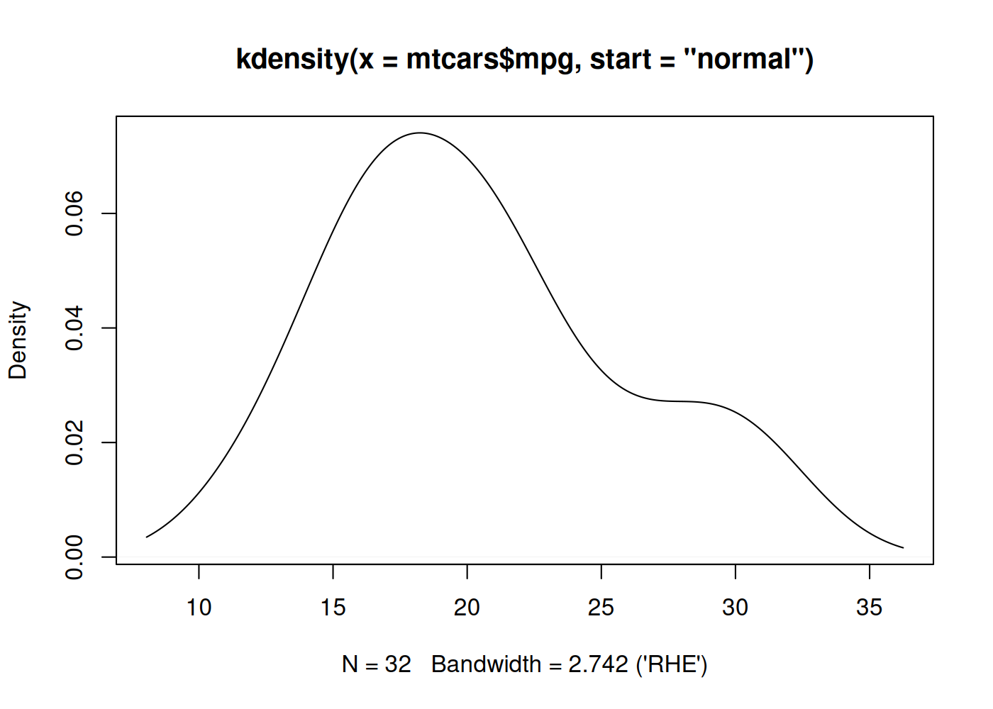
plot(kdensity(mtcars$mpg, start = "normal"))
Description
A parametric start (Hjort and Glad, 1995) fits a parametric density first and uses kernel density estimation to correct it. When the true density is close to the start, this beats the ordinary kernel density estimator, and it often does well even when the start is some way off.
Asymmetric kernels avoid boundary bias for data on the unit interval
or the positive half-line. kdensity has Jones and Henderson’s Gaussian
copula kernel (gcopula), Chen’s beta kernels (beta, beta_biased),
and Chen’s gamma kernels (gamma, gamma_biased). Starts and kernels
can be combined, as in the example below.
Usage
The function kdensity takes some data, a kernel kernel and a
parametric start start. You can optionally specify the support
parameter, which is used to find the normalizing constant.
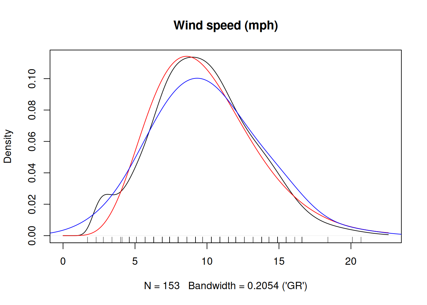
The following example uses the datasets::airquality data set. The
black curve is a gamma-kernel density estimate with a gamma start, the
red curve a fully parametric gamma density, and the blue curve an
ordinary density estimate. Notice the boundary bias of the ordinary
density estimator. The underlying parameter estimates are always
maximum likelihood.
library("kdensity")
kde <- kdensity(airquality$Wind, start = "gamma", kernel = "gamma")
plot(kde, main = "Wind speed (mph)")
lines(kde, plot_start = TRUE, col = "red")
lines(density(airquality$Wind, adjust = 2), col = "blue")
rug(airquality$Wind)
Since the return value of kdensity is a function, kde is callable
and can be used as any density function in R (such as stats::dnorm).
For example, you can do:
kde(10)
#> [1] 0.1101274
integrate(kde, lower = 0, upper = 1) # The cumulative distribution up to 1.
#> 9.499222e-06 with absolute error < 1.5e-11
For large plotting grids, kdensity_grid() provides an explicitly
approximate binning-and-FFT backend for every built-in symmetric kernel
and the Gaussian-copula kernel. Calling kde() remains exact.
You can access the parameter estimates by using coef. You can also
access the log likelihood (logLik), AIC and BIC of the parametric
start distribution.
coef(kde)
#> Maximum likelihood estimates for the Gamma model
#>  shape    rate
#> 7.1873  0.7218
logLik(kde)
#> 'log Lik.' -410.5129 (df=2)
AIC(kde)
#> [1] 825.0259