Small Area Estimation Hierarchical Bayes for Spatial Beta Model

Provides several functions and datasets for area-level Small Area Estimation using the Hierarchical Bayesian (HB) method. Model-based estimators are designed for variables of interest that follow a Beta distribution (proportions bounded between 0 and 1). The package supports both non-spatial and spatial models based on Simultaneous Autoregressive (SAR) and Leroux Conditional Autoregressive (CAR) structures for area-level random effects, with optional survey design effect (DEFF) adjustments for sampling variances. In addition, it provides utility functions for constructing spatial weights matrices and performing spatial autocorrelation diagnostics. The 'runjags' package is used to obtain posterior estimates via Markov Chain Monte Carlo (MCMC) with parallel computing capabilities. For references, see Rao and Molina (2015) , Liu et al. (2014) < https://www150.statcan.gc.ca/n1/pub/12-001-x/2014001/article/14030-eng.pdf>, Kubacki and Jedrzejczak (2016) , Leroux et al. (2000) , Chung and Datta (2020) < https://www.census.gov/content/dam/Census/library/working-papers/2020/adrm/RRS2020-07.pdf>, Figueroa-Zúñiga et al. (2013) , Denwood (2016) , Anselin (1988) , and Anselin and Morrison (2019) < https://spatialanalysis.github.io/lab_tutorials/Spatial_Weights_as_Distance_Functions.html>.

saeHB.Spatial.Beta

The saeHB.Spatial.Beta package provides several functions to estimate small area proportions using the Hierarchical Bayesian (HB) method. Model-based estimators are designed for variables of interest that follow a Beta distribution (proportions bounded between 0 and 1). The package supports both non-spatial and spatial models based on Simultaneous Autoregressive (SAR) and Leroux Conditional Autoregressive (CAR) structures for area-level random effects, with optional survey design effect (DEFF) adjustments for sampling variances. In addition, it provides utility functions for constructing spatial weights matrices and performing spatial autocorrelation diagnostics. The runjags package is used to obtain posterior estimates via Markov Chain Monte Carlo (MCMC) with parallel computing capabilities.

Author

Boby Iwan, Cucu Sumarni

Maintainer

Boby Iwan [email protected]

Functions

• betadeff_sar() Estimates small area proportions using a Hierarchical Bayes (HB) method under a Spatial SAR Model with a Beta distribution, incorporating survey design effect (DEFF) adjustments.
• beta_sar() Estimates small area proportions using a Hierarchical Bayes (HB) method under a Spatial SAR Model with a Beta distribution without DEFF adjustments, by estimating the unknown precision parameter.
• betadeff_lerouxcar() Estimates small area proportions using a Hierarchical Bayes (HB) method under a Spatial Leroux CAR Model with a Beta distribution, incorporating survey design effect (DEFF) adjustments.
• beta_lerouxcar() Estimates small area proportions using a Hierarchical Bayes (HB) method under a Spatial Leroux CAR Model with a Beta distribution without DEFF adjustments, by estimating the unknown precision parameter.
• betadeff_nonspatial() Estimates small area proportions using a Hierarchical Bayes (HB) method under a Non-Spatial Model with a Beta distribution and Independent and Identically Distributed (IID) random effects, incorporating DEFF adjustments.
• beta_nonspatial() Estimates small area proportions using a Hierarchical Bayes (HB) method under a Non-Spatial Model with a Beta distribution and IID random effects without DEFF adjustments, by estimating the unknown precision parameter.
• build_w() A utility function to construct spatial weights matrices (contiguity, distance, or kernel) required for spatial modeling.
• moran_test() A diagnostic function to perform Moran’s I test for spatial autocorrelation.

Installation

System Requirement: Since this package relies on runjags for parallel MCMC computations, you must first install the JAGS (Just Another Gibbs Sampler) software on your computer before installing this package.

You can install the development version of saeHB.Spatial.Beta from GitHub with:

# install.packages("devtools")
devtools::install_github("BobyIwan/saeHB.Spatial.Beta")

Or, to include the vignette, use the following command:

devtools::install_github("BobyIwan/saeHB.Spatial.Beta", build_vignettes = TRUE)

Example

This is a basic example of using the betadeff_sar() function to make an estimate based on synthetic data in this package:

library(saeHB.Spatial.Beta)

# Load dataset and proximity matrix
data(databeta)
data(weight_mat)

# Fitting the Spatial SAR model
model_sar_deff <- betadeff_sar(
  formula = y ~ x1 + x2,
  deff = "deff",
  n_i = "n_i",
  proxmat = weight_mat,
  data = databeta
)

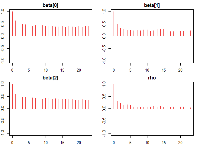
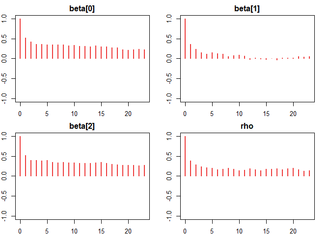
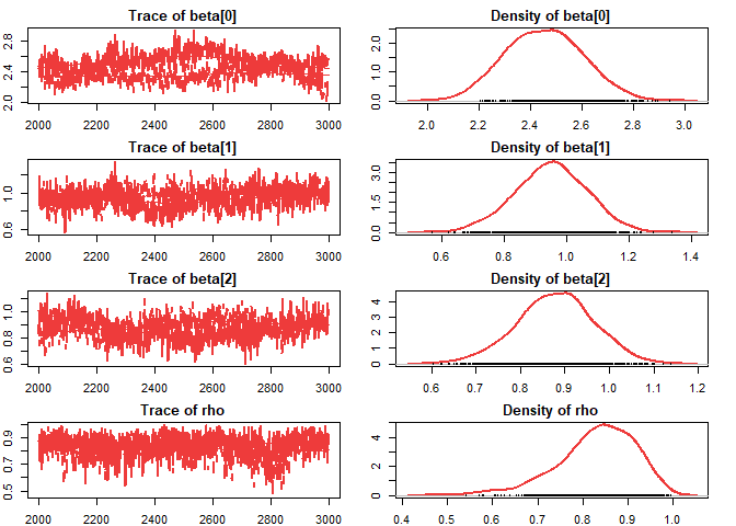
Extract the mean estimation for the areas:

head(model_sar_deff$est)
#>        Estimate   Est.Error  l-95% CI  u-95% CI
#> mu[1] 0.6566512 0.125923984 0.4326561 0.8526547
#> mu[2] 0.6963246 0.071163943 0.5509475 0.8327443
#> mu[3] 0.8444858 0.051630642 0.7286889 0.9175998
#> mu[4] 0.8971752 0.042525156 0.7983507 0.9631127
#> mu[5] 0.9098190 0.059951310 0.7579548 0.9750523
#> mu[6] 0.9964128 0.002605478 0.9890639 0.9991400

Extract the estimated model coefficients:

model_sar_deff$coefficient
#>          Estimate  Est.Error  l-95% CI  u-95% CI     Rhat       ESS
#> beta[0] 2.4520550 0.14851860 2.1757003 2.7440245 2.156080  59.39028
#> beta[1] 0.9494867 0.11249428 0.7214834 1.1657507 1.041024 304.63867
#> beta[2] 0.8786401 0.08584050 0.7012405 1.0430313 1.074113  51.10860
#> rho     0.8316615 0.08489129 0.6256059 0.9671044 1.082723 400.02518

Extract the random effect for the areas:

model_sar_deff$randeff
#>          Estimate Est.Error    l-95% CI   u-95% CI
#> v[1]  -2.01472185 0.6372259 -3.03530350 -0.9558320
#> v[2]  -0.93610269 0.3811039 -1.70014000 -0.1453370
#> v[3]  -0.75376238 0.4415716 -1.73914000  0.0187899
#> v[4]   0.70167832 0.5075260 -0.27024605  1.7731467
#> v[5]   1.29966801 0.5994045  0.09466170  2.4694800
#> v[6]   1.45934311 0.6599842  0.18714100  2.6722100
#> v[7]  -2.73458282 0.3677825 -3.57728025 -2.0344200
#> v[8]  -2.72768875 0.3158727 -3.27246000 -2.0864100
#> v[9]  -0.73968440 0.4693168 -1.53919000  0.1433260
#> v[10]  0.26730882 0.6920880 -0.99071700  1.7570200
#> v[11]  1.84688703 0.3875205  1.12734000  2.6195800
#> v[12]  1.14933151 0.4750051  0.18962567  2.1107900
#> v[13] -1.45559410 0.5371914 -2.42973775 -0.3801220
#> v[14] -1.57087936 0.5142320 -2.54021575 -0.6089981
#> v[15] -1.19285455 0.5238957 -2.16357750 -0.2338669
#> v[16]  0.64101829 0.4936966 -0.28630700  1.6237500
#> v[17]  1.84123011 0.5041058  0.94713300  2.9795300
#> v[18]  1.47853613 0.5544432  0.49294000  2.6089300
#> v[19] -1.01471208 0.5629174 -2.12719000 -0.0104731
#> v[20] -0.75083646 0.3979580 -1.59001000 -0.0177030
#> v[21] -0.24138545 0.5824161 -1.16030000  1.1180500
#> v[22] -0.08830559 0.4804839 -0.79445900  1.3822200
#> v[23]  1.48098675 0.5897468  0.41117395  2.9039600
#> v[24]  1.16027949 0.4825320  0.09255001  2.0324300
#> v[25] -1.15534168 0.4739891 -2.10702000 -0.2856152
#> v[26] -0.05308789 0.4675652 -1.01282000  0.7197088
#> v[27]  0.07922888 0.8443436 -1.34420000  1.7782300
#> v[28]  0.80096625 0.5096009 -0.01340528  1.9523400
#> v[29]  0.70576451 0.5338296 -0.36324000  1.7655792
#> v[30]  1.02251378 0.5836198 -0.07398682  2.1411800
#> v[31] -0.16187577 0.5182311 -1.06493700  0.9899240
#> v[32] -0.12876429 0.5088627 -0.99675900  0.8548070
#> v[33] -0.01825535 0.4310696 -0.78959918  0.8954781
#> v[34]  0.34941414 0.3690757 -0.53742600  1.0887222
#> v[35]  2.23577497 0.5365541  1.07893350  3.5891475
#> v[36]  1.05534037 0.6843919 -0.38907200  2.2636900

Extract the random effect variance for the areas:

model_sar_deff$refvar
#>           Estimate Est.Error  l-95% CI u-95% CI
#> a.var[1]  4.274875  20.90236 0.9593703 17.31051
#> a.var[2]  4.193587  20.96965 0.9217799 17.17273
#> a.var[3]  3.972008  20.97843 0.8600865 16.48555
#> a.var[4]  3.972008  20.97843 0.8600865 16.48555
#> a.var[5]  4.193587  20.96965 0.9217799 17.17273
#> a.var[6]  4.274875  20.90236 0.9593703 17.31051
#> a.var[7]  4.193587  20.96965 0.9217799 17.17273
#> a.var[8]  4.152950  21.08749 0.8927992 17.23302
#> a.var[9]  3.932631  21.09825 0.8319131 16.53811
#> a.var[10] 3.932631  21.09825 0.8319131 16.53811
#> a.var[11] 4.152950  21.08749 0.8927992 17.23302
#> a.var[12] 4.193587  20.96965 0.9217799 17.17273
#> a.var[13] 3.972008  20.97843 0.8600865 16.48555
#> a.var[14] 3.932631  21.09825 0.8319131 16.53811
#> a.var[15] 3.757189  21.12101 0.7789302 16.10273
#> a.var[16] 3.757189  21.12101 0.7789302 16.10273
#> a.var[17] 3.932631  21.09825 0.8319131 16.53811
#> a.var[18] 3.972008  20.97843 0.8600865 16.48555
#> a.var[19] 3.972008  20.97843 0.8600865 16.48555
#> a.var[20] 3.932631  21.09825 0.8319131 16.53811
#> a.var[21] 3.757189  21.12101 0.7789302 16.10273
#> a.var[22] 3.757189  21.12101 0.7789302 16.10273
#> a.var[23] 3.932631  21.09825 0.8319131 16.53811
#> a.var[24] 3.972008  20.97843 0.8600865 16.48555
#> a.var[25] 4.193587  20.96965 0.9217799 17.17273
#> a.var[26] 4.152950  21.08749 0.8927992 17.23302
#> a.var[27] 3.932631  21.09825 0.8319131 16.53811
#> a.var[28] 3.932631  21.09825 0.8319131 16.53811
#> a.var[29] 4.152950  21.08749 0.8927992 17.23302
#> a.var[30] 4.193587  20.96965 0.9217799 17.17273
#> a.var[31] 4.274875  20.90236 0.9593703 17.31051
#> a.var[32] 4.193587  20.96965 0.9217799 17.17273
#> a.var[33] 3.972008  20.97843 0.8600865 16.48555
#> a.var[34] 3.972008  20.97843 0.8600865 16.48555
#> a.var[35] 4.193587  20.96965 0.9217799 17.17273
#> a.var[36] 4.274875  20.90236 0.9593703 17.31051

References

• Rao, J. N. K., & Molina, I. (2015). Small Area Estimation (2nd ed.). New Jersey: John Wiley & Sons, Inc. doi:10.1002/9781118735855.
• Liu, B., Lahiri, P., & Kalton, G. (2014). Hierarchical Bayes Modeling of Survey-Weighted Small Area Proportions. Statistics Canada. https://www150.statcan.gc.ca/n1/pub/12-001-x/2014001/article/14030-eng.pdf.
• Kubacki, J., & Jedrzejczak, A. (2016). Small Area Estimation of Income Under Spatial SAR Model. Statistics in Transition New Series, 17(3), 365–390. doi:10.59170/stattrans-2016-022.
• Leroux, B. G., Lei, X., & Breslow, N. (2000). Estimation of Disease Rates in Small Areas: A New Mixed Model for Spatial Dependence. In M. E. Halloran & D. Berry (Eds.), Statistical Models in Epidemiology, the Environment, and Clinical Trials (Vol. 116, pp. 179–191). New York: Springer. doi:10.1007/978-1-4612-1284-3_4.
• Chung, H. C., & Datta, G. S. (2020). Bayesian Hierarchical Spatial Models for Small Area Estimation (Research Report Series). Washington, D.C.: U.S. Census Bureau. https://www.census.gov/content/dam/Census/library/working-papers/2020/adrm/RRS2020-07.pdf.
• Figueroa-Zúñiga, J. I., Arellano-Valle, R. B., & Ferrari, S. L. P. (2013). Mixed beta regression: A Bayesian perspective. Computational Statistics & Data Analysis, 61, 137-147. doi:10.1016/j.csda.2012.12.002.
• Denwood, M. J. (2016). runjags: An R Package Providing Interface Utilities, Model Templates, Parallel Computing Methods and Additional Distributions for MCMC Models in JAGS. Journal of Statistical Software, 71(9), 1–25. doi:10.18637/jss.v071.i09.
• Anselin, L. (1988). Spatial Econometrics: Methods and Models. Dordrecht: Springer Netherlands. doi:10.1007/978-94-015-7799-1.
• Anselin, L., & Morrison, S. (2019). Spatial Weights as Distance Functions. https://spatialanalysis.github.io/lab_tutorials/Spatial_Weights_as_Distance_Functions.html.