Tidyverse-Based Reliability and Survival Data Visualization Tool

A suite of reliability/survival data visualization tools that leverage the Tidyverse Grammar of Graphics. Time-based aesthetics may be specified alongside standard non-aesthetic arguments to generate highly customizable graphs.

surviveR

The surviveR package is a reliability and survival data visualization tool that leverages the user-friendliness of the Tidyverse ecosystem. Functions in surviveR allow users to specify time-based aesthetics alongside standard non-aesthetic arguments to generate highly customizable graphs.

Installation

The surviveR package is currently under review for inclusion in the CRAN repository. In the meantime, you can install the development version of surviveR via one of 2 methods–the remotes package (probably the easiest) or downloading the files directly from the GitHub.

Option 1: the remotes package (if you already have a Github account)

# install.packages("remotes")
# 
# library(remotes)
# 
# remotes::install_github("KLGORE/surviveR")
# 
# library(surviveR)

Option 2: Download directly from GitHub

If downloading the package files directly from GitHub, please follow these steps:

1. Click on (this link)[https://github.com/KLGORE/surviveR] and and download all package files into a folder on your computer.

2. Open up an R session and set your working directory to the path to the folder that contains all of the package files.

3. Make sure the following packages are installed and loaded on your computer: tidyverse, devtools, survival, and flexsurv. (I’m reasonably sure these get automatically installed and loaded with the installation, but if you run into issues installing the package, try loading those packages and try again.)

4. Run load_all() in your console. Then you should have full access to the wonders of surviveR!

Package contents

The current version of surviveR features data visualizations for the following survival plots:

• Kaplan-Meier (KM) plot

• Cox Proportional Hazards (CoxPH) plot

• Parametric survival plot

• Weibull plot

• Mean Cumulative Function (MCF) plot

Users may specify whether they want to visualize the survival probability or cumulative failure probability in the arguments. Additionally, each geom_[fill in the blank] comes in 2 “flavors”–one in which the user specifies the time and grouping variables in the aesthetics mapping and one in which they are specified via a survival formula.

Sample datasets

This package features two pre-loaded simulated datasets–mfg and device_repair.

The mfg dataset contains data from a fictional reliability pilot study in which 150 customers receive one of two device types (“A” or “B”). The manufacturing location of each device is recorded in the mfg_location variable (“CA”, “OR”, or “WA”). The time to failure ttf variable is the time variable of interest. Values of 1 in the status column indicate no censoring, whereas values of 1 indicate right censoring.

The mfg dataset is used to demonstrate capabilities of the geom_km, geom_coxph, geom_survreg, and geom_weibull functions.

head(mfg,20)
#> # A tibble: 20 × 7
#>    device_id mfg_location device_type pilot_start status end_date     ttf
#>    <chr>     <chr>        <chr>       <date>       <dbl> <date>     <dbl>
#>  1 WBOEX558  OR           A           2023-01-01       1 2023-03-07    65
#>  2 KDEYG321  CA           A           2023-01-01       1 2023-01-19    18
#>  3 GVDAG267  WA           A           2023-01-01       1 2023-02-13    43
#>  4 KSIXB271  CA           B           2023-01-01       1 2023-03-05    63
#>  5 ZYXWI609  CA           B           2023-01-01       1 2023-03-25    83
#>  6 TPOTI226  OR           B           2023-01-01       0 2023-04-01    90
#>  7 OTVYQ973  WA           A           2023-01-01       1 2023-03-05    63
#>  8 YKAAK334  CA           B           2023-01-01       1 2023-03-21    79
#>  9 RPECL230  WA           A           2023-01-01       1 2023-01-17    16
#> 10 KLKBF575  WA           B           2023-01-01       1 2023-02-26    56
#> 11 XAHMV390  WA           B           2023-01-01       0 2023-04-01    90
#> 12 KDHIQ074  CA           B           2023-01-01       1 2023-03-28    86
#> 13 TEPWK136  CA           A           2023-01-01       1 2023-01-20    19
#> 14 YYMIN719  CA           B           2023-01-01       0 2023-04-01    90
#> 15 CGOXI217  CA           A           2023-01-01       1 2023-01-09     8
#> 16 MWEVJ903  CA           B           2023-01-01       1 2023-03-29    87
#> 17 LHTZA745  OR           B           2023-01-01       1 2023-03-03    61
#> 18 DZJAC890  OR           A           2023-01-01       1 2023-01-14    13
#> 19 NMZBZ716  CA           B           2023-01-01       1 2023-02-28    58
#> 20 STZVA513  CA           B           2023-01-01       0 2023-04-01    90

The device_repair dataset showcases fictional multi-event data for a fictional device. The device_id column contains unique identifiers for each device, with the repair_time column indicating the time in which an event (failure or device retirement) occurred. Regardless of the presence of a status column, the maximum event time for each device_id is assumed to be the censoring time for the device.

The device_repair dataset is used to showcase the capabilities of geom_mcf, which visualizes the mean cumulative function (MCF) for repairable systems.

head(device_repair,20)
#> # A tibble: 20 × 5
#>    device_id repair_time status device_type mfg_location
#>    <chr>           <dbl>  <dbl> <chr>       <chr>       
#>  1 MKFGQ650           93      1 A           OR          
#>  2 MKFGQ650          101      0 A           OR          
#>  3 GVDAG267          562      0 A           OR          
#>  4 IVRHK669           60      1 A           CA          
#>  5 IVRHK669           61      1 A           CA          
#>  6 IVRHK669           69      1 A           CA          
#>  7 IVRHK669           78      0 A           CA          
#>  8 ZWYTN953           82      1 A           OR          
#>  9 ZWYTN953           96      1 A           OR          
#> 10 ZWYTN953          113      1 A           OR          
#> 11 ZWYTN953          125      1 A           OR          
#> 12 ZWYTN953          139      1 A           OR          
#> 13 ZWYTN953          156      0 A           OR          
#> 14 ORLZJ057          382      1 A           OR          
#> 15 ORLZJ057          391      1 A           OR          
#> 16 ORLZJ057          393      1 A           OR          
#> 17 ORLZJ057          404      1 A           OR          
#> 18 ORLZJ057          418      1 A           OR          
#> 19 ORLZJ057          428      1 A           OR          
#> 20 ORLZJ057          432      0 A           OR

Survival functions

The following sections provide a preview of the capabilities of the surviveR package. Each subsection contains examples for how to generate the same plot by specifying variables through the aesthetics mapping or a formula.

For more details, please reference the documentation.

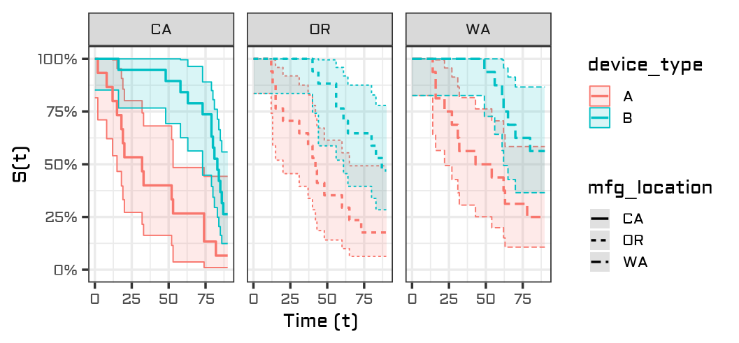
Nonparametric: Kaplan-Meier curves

geom_km

my_plot=
mfg %>% 
     ggplot() +
     geom_km(aes(time = ttf, time2 = status, treatments = device_type, strata = mfg_location)) +
     facet_grid(.~mfg_location)

geom_km2 (formula-based input)

my_plot=
mfg %>% 
     ggplot() +
     geom_km2( Surv(ttf, status) ~ device_type + strata(mfg_location) ) +
     facet_grid(.~mfg_location)

Resulting plot:

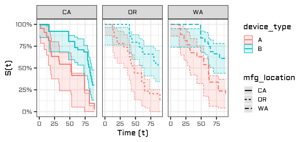
Semiparametric: Cox Proportional Hazards curves

geom_coxph

my_plot=
mfg %>% 
     ggplot() +
     geom_coxph(aes(time = ttf, time2 = status, treatments = device_type, strata = mfg_location)) +
     facet_grid(.~mfg_location)

geom_coxph2

my_plot=
mfg %>% 
     ggplot() +
     geom_coxph2( Surv(ttf, status) ~ device_type + strata(mfg_location) ) +
     facet_grid(.~mfg_location)

Resulting plot:

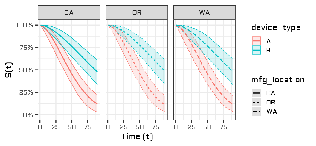
Parametric regression curves

geom_survreg

my_plot=
mfg %>% 
     ggplot() +
     geom_survreg(aes(time = ttf, time2 = status, treatments = device_type, strata = mfg_location)) +
     facet_grid(.~mfg_location)

geom_survreg2

my_plot=
mfg %>% 
     ggplot() +
     geom_survreg2( Surv(ttf, status) ~ device_type + strata(mfg_location) ) +
     facet_grid(.~mfg_location)

Resulting plot:

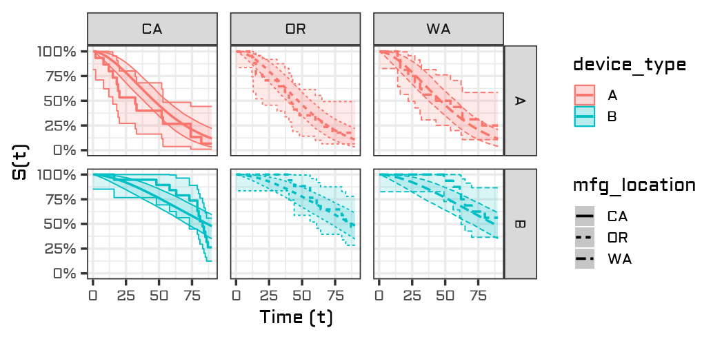
Overlaying Fits

Layers with aesthetics mapping

my_plot=
mfg %>%
    ggplot() +
    geom_survreg(
     aes(time=ttf, time2=status, trt=device_type, strata=mfg_location)
    ) +
    geom_km() +
    facet_grid(device_type ~ mfg_location, scale="free_x")

Resulting plot:

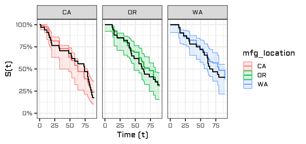
Layers with formulas

my_plot=
mfg %>%
    ggplot() +
    geom_coxph2(Surv(ttf,status)~mfg_location) +
    geom_km2(color="black", conf.int=F) +
    facet_grid(.~mfg_location)

Resulting plot:

Other

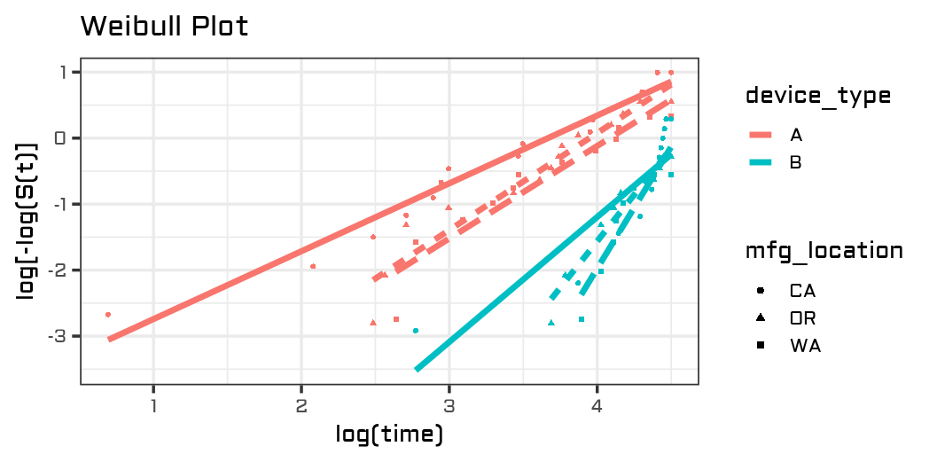
Weibull plots

my_plot=mfg %>% 
     ggplot() +
     geom_weibull(aes(time = ttf, time2 = status, treatments = device_type, strata = mfg_location))

Resulting plot:

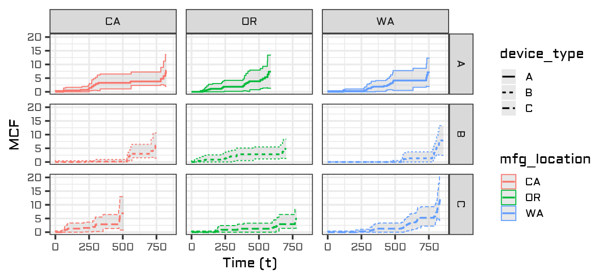
Mean Cumulative Function (MCF) Plots

my_plot=
device_repair %>%
    ggplot()+
    geom_mcf(
        aes(time = repair_time, ids = device_id, trt = mfg_location, strata = device_type),
        conf.fill = "gray", conf.alpha = 0.35) +
    facet_grid(device_type~mfg_location)

Resulting plot:

In the works

The following functions are in varying stages of development:

• geom_event - for visualizing event plots (was previously available, but we decided to take it offline to make changes to the layering scheme)

• geom_ALT_temp - for visualizing Arrhenius-accelerated data from accelerated life tests (ALT’s)

• geom_ALT_volt - for visualizing voltage-accelerated data from accelerated life tests (ALT’s)

Stay tuned!